Apode Tutorial

This tutorial shows the current functionalities of the Apode package. Apode contains various methods to calculate measures and generate graphs on the following topics:

• Poverty

• Inequality

• Welfare

• Polarization

• Concentration

Getting Started

ApodeData class

The objects are created as:

ad = ApodeData(DataFrame,income_column)

Where income_column is the name of the column of interest for the analysis in the dataframe.

Methods that calculate indicators:

ad.poverty(method,*args)
ad.ineq(method,*args)
ad.welfare(method,*args)
ad.polarization(method,*args)
ad.concentration(method,*args)

Métodos that generate graphs:

ad.plot.hist()
ad.plot.tip(**kwargs)
ad.plot.lorenz(**kwargs)
ad.plot.pen(**kwargs)

For an introduction to the Python language see Beginner Guide.

Data Creation and Description

• Data can be generated manually or by means of a simulation. They are contained in a DataFrame object.

• Other categoric variables that allow for the indicators to be applied by groups (groupby) might be available.

import numpy as np
import pandas as pd

from apode import ApodeData
from apode import datasets

Manual data loading

An object can be generated from a DataFrame or from a valid argument in the DataFrame method.

x = [23, 10, 12, 21, 4, 8, 19, 15, 11, 9]
df1 = pd.DataFrame({'x':x})
ad1 = ApodeData(df1, income_column="x")
ad1

	x
0	23
1	10
2	12
3	21
4	4
5	8
6	19
7	15
8	11
9	9

ApodeData(income_column='x') - 10 rows x 1 columns

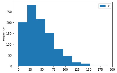
Data simulation

The module datasets contains some distribution examples commonly used to model the income distribution. For example:

# Generate data
n = 1000 # observations
seed = 12345
ad2 = datasets.make_weibull(seed=seed,size=n)
ad2.describe()

	x
count	1000.000000
mean	45.408376
std	30.207372
min	0.112876
25%	22.363891
50%	39.404779
75%	62.690946
max	190.596705

# Plotting the distribution
ad2.plot();

Other distributions are: uniform, lognormal, exponential, pareto, chisquare and gamma. For help type:

help(datasets.make_weibull)

Help on function make_weibull in module apode.datasets:

make_weibull(seed=None, size=100, a=1.5, c=50, nbin=None)
    Weibull Distribution.

    Parameters
    ----------
    seed: int, optional(default=None)

    size: int, optional(default=100)

    a: float, optional(default=1.5)

    c: float, optional(default=50)

    nbin: int, optional(default=None)

    Return
    ------
    out: float array
        Array of random numbers.

Poverty

The following poverty measures are implemented:

• headcount: Headcount Index

• gap: Poverty gap Index

• severity: Poverty Severity Index

• fgt: Foster–Greer–Thorbecke Indices

• sen: Sen Index

• sst: Sen-Shorrocks-Thon Index

• watts: Watts Index

• cuh: Clark, Ulph and Hemming Indices

• takayama: Takayama Index

• kakwani: Kakwani Indices

• thon: Thon Index

• bd: Blackorby and Donaldson Indices

• hagenaars: Hagenaars Index

• chakravarty: Chakravarty Indices

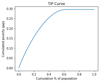
Also the TIP curve, which allows for a graphic comparison of poverty amongst different distributions.

Numerical measures

All the methods require the poverty line (pline) as argument for get a absolute measure of poverty.

pline = 50 # Poverty line
p = ad2.poverty('headcount',pline=pline)
p

0.626

If the argument is omitted 0.5*median is used. Other options for a relative measure of poverty are:

# pline = factor*stat  [stat: mean, median, quantile_q]
p1 = ad2.poverty('headcount')  # pline= 0.5*median(y)
p2 = ad2.poverty('headcount', pline='median', factor=0.5)
p3 = ad2.poverty('headcount', pline='quantile', q=0.5, factor=0.5)
p4 = ad2.poverty('headcount', pline='mean', factor=0.5)
p1, p2, p3, p4

(0.214, 0.214, 0.214, 0.256)

Some methods require an additional parameter, alpha. In some cases, a default value is set for it. The summary function shows the result of various methods:

df_p = poverty_summary(ad2)
df_p

	method	measure
0	headcount	0.214000
1	gap	0.088038
2	severity	0.052488
3	fgt(1.5)	0.066208
4	sen	0.134042
5	sst	0.164471
6	watts	0.155405
7	cuh(0)	0.917773
8	cuh(0.5)	0.112144
9	takayama	0.083811
10	kakwani	0.139643
11	thon	0.164395
12	bd(1.0)	0.110478
13	bd(2.0)	0.158095
14	hagenaars	0.052136
15	chakravarty(0.5)	0.056072

Graph measures

# TIP curve
ad2.plot.tip(pline=pline);

Exercise: Comparison of poverty measures

In this exercise some properties of three poverty measures are compared: headscount, poverty gap and severity index (they are part of the FGT class). The exercise compares three distributions:

x1 = np.array([5,20,35,60])
x2 = x1 +  np.array([10, 10, 10, 0])
x3 = x2 +  np.array([10,0,-10, 0])
dfe = pd.DataFrame({'x1':x1,'x2':x2,'x3':x3})
dfe

	x1	x2	x3
0	5	15	25
1	20	30	30
2	35	45	35
3	60	60	60

pline = 50
ade1 = ApodeData(dfe,income_column='x1')
ade2 = ApodeData(dfe,income_column='x2')
ade3 = ApodeData(dfe,income_column='x3')

# Headcount
ade1.poverty('headcount',pline=pline), ade2.poverty('headcount',pline=pline), ade3.poverty('headcount',pline=pline)

(0.75, 0.75, 0.75)

The greatest virtues of the headcount index are that it is simple to construct and easy to understand. However, the measure does not take the intensity of poverty into account (the three indices are equal).

# Poverty Gap
ade1.poverty('gap',pline=pline), ade2.poverty('gap',pline=pline), ade3.poverty('gap',pline=pline)

(0.45, 0.30000000000000004, 0.3)

The poverty gap index gives an idea of the cost to eliminate poverty (in relation to the poverty line). But the previous indices are unsatisfactory because they violate the transfer principle which states that transfers from a richer person to a poorer person should improve the welfare measure (x2 versus x3). This property is captured by the severity index.

# Severity
ade1.poverty('severity',pline=pline), ade2.poverty('severity',pline=pline), ade3.poverty('severity',pline=pline)

(0.315, 0.16499999999999998, 0.125)

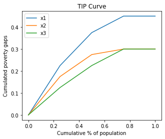
TIP curves are cumulative poverty gap curves used for representing the three different aspects of poverty: incidence, intensity and inequality (severity). Non-intersection of TIP curves is recognized as a criterion to compare income distributions in terms of poverty.

ax = ade1.plot.tip(pline=pline)
ade2.plot.tip(ax=ax, pline=pline)
ade3.plot.tip(ax=ax, pline=pline)
ax.legend(['x1','x2','x3']);

Exercise: Contribution of each subgroup to aggregate poverty

Another convenient feature of the FGT class of poverty measures is that they can be disaggregated for population subgroups and the contribution of each subgroup to aggregate poverty can be calculated. For instance:

x = [23, 10, 12, 21, 4, 8, 19, 15, 5, 7]
y = [10,10,20,10,10,20,20,20,10,10]
region = ['urban','urban','rural','urban','urban','rural','rural','rural','urban','urban']
dfa = pd.DataFrame({'x':x,'region':region})
ada1 = ApodeData(dfa,income_column='x')
ada1

	x	region
0	23	urban
1	10	urban
2	12	rural
3	21	urban
4	4	urban
5	8	rural
6	19	rural
7	15	rural
8	5	urban
9	7	urban

ApodeData(income_column='x') - 10 rows x 2 columns

# group calculation according to variable "y"
pline = 11
pg = poverty_groupby(ada1,'headcount',group_column='region', pline=pline)
pg

	x_measure	x_weight
rural	0.250000	4
urban	0.666667	6

# simple calculation
ps = ada1.poverty('headcount',pline=pline)
ps

0.5

# If the indicator is decomposable, the same result is attained:
pg_p = sum(pg['x_measure']*pg['x_weight']/sum(pg['x_weight']))
pg_p

0.5

Inequality

The following inequality measures are implemented:

• gini: Gini Index

• entropy: Generalized Entropy Index

• atkinson: Atkinson Index

• rrange: Relative Range

• rad: Relative average deviation

• cv: Coefficient of variation

• sdlog: Standard deviation of log

• merhan: Merhan index

• piesch: Piesch Index

• bonferroni: Bonferroni Indices

• kolm: Kolm Index

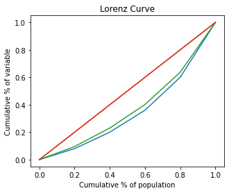
Also the Lorenz and Pen curves, which allows for a graphic comparison of inequality among different distributions.

Numerical measures

# Evaluate an inequality method
q = ad2.inequality('gini')
q

0.3652184907296814

The summary function shows the result of various methods:

df_ineq = inequality_summary(ad2)
df_ineq

	method	measure
0	rrange	4.194905
1	rad	0.264575
2	cv	0.664905
3	sdlog	0.916263
4	gini	0.365218
5	merhan	0.512500
6	piesch	0.288587
7	bonferroni	0.510418
8	kolm(0.5)	36.566749
9	ratio(0.05)	0.032061
10	ratio(0.2)	0.118795
11	entropy(0)	0.281897
12	entropy(1)	0.217586
13	entropy(2)	0.221049
14	atkinson(0.5)	0.114579
15	atkinson(1.0)	0.245649
16	atkinson(2.0)	0.631276

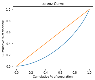
Graph measures

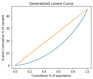
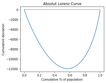
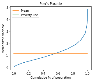
The relative, generalized and absolute Lorenz Curves are implemented. Alse de Pen Parade curve.

# Lorenz Curves
ad2.plot.lorenz();

# Generalized Lorenz Curve
ad2.plot.lorenz(alpha='g');

# Absolute Lorenz Curve
ad2.plot.lorenz(alpha='a');

# Pen's Parade
ad2.plot.pen(pline=60);

Exercise: Redistributive Effect of Fiscal Policy

Income pre and post fiscal policy:

# Income pre fiscal policy:
y_pre = np.array([20, 30, 40, 60, 100])

# Fiscal policy
tax = 0.2*np.maximum(y_pre-35,0)  # tax formula
revenue = np.sum(tax)             # total revenue
transfers = revenue/len(y_pre)    # per capita transfers

# Income post fiscal policy:
y_post = y_pre - tax + transfers

# ApodeData
df_pre = pd.DataFrame({'y1':y_pre})
ad_pre = ApodeData(df_pre,income_column='y1')

df_post = pd.DataFrame({'y2':y_post})
ad_post = ApodeData(df_post,income_column='y2')
ad_post

	y2
0	23.8
1	33.8
2	42.8
3	58.8
4	90.8

ApodeData(income_column='y2') - 5 rows x 1 columns

# Gini
ad_pre.inequality.gini(), ad_post.inequality.gini()  # decrease inequality

(0.30399999999999994, 0.25440000000000024)

# Lorenz Curves
ax = ad_pre.plot.lorenz()
ad_post.plot.lorenz(ax=ax);

Welfare

The following welfare measures are implemented:

• utilitarian: Utilitarian utility function

• rawlsian: Rawlsian utility function

• isoelastic: Isoelastic utility function

• sen: Sen utility function

• theill: Theill utility function

• theilt: Theilt utility function

# Evaluate a welfare method
w = ad2.welfare('sen')
w

28.824397753868958

The summary function shows the result of various methods:

df_wlf = welfare_summary(ad2)
df_wlf

	method	measure
0	utilitarian	45.408376
1	rawlsian	0.112876
2	sen	28.824398
3	theill	34.253866
4	theilt	36.529160
5	isoelastic(0)	45.408376
6	isoelastic(1)	3.533799
7	isoelastic(2)	-0.059726
8	isoelastic(inf)	0.112876

Polarization

The following welfare measures are implemented:

• ray: Esteban and Ray index

• wolfson: Wolfson index

# Evaluate a polarization method
p = ad2.polarization('ray')
p

0.03316795744715791

The summary function shows the result of various methods:

df_pz = polarization_summary(ad2)
df_pz

	method	measure
0	ray	0.033168
1	wolfson	0.357081

Concentration

The following concentration measures are implemented:

• herfindahl: Herfindahl-Hirschman Index

• rosenbluth: Rosenbluth Index

• concentration_ratio: Concentration Ratio Index

# Evaluate a concentration method
c = ad2.concentration('herfindahl')
c

0.00044254144331556705

The summary function shows the result of various methods:

df_conc = concentration_summary(ad2)
df_conc

	method	measure
0	herfindahl	0.000443
1	herfindahl(norm)	0.000443
2	rosenbluth	0.001575
3	concentration_ratio(1)	0.004197
4	concentration_ratio(3)	0.010900

References

Schröder, C. (2011). Cowell, F.: Measuring Inequality. London School of Economics Perspectives in Economic Analysis.

Adler, M. D., & Fleurbaey, M. (Eds.). (2016). The Oxford handbook of well-being and public policy. Oxford University Press.

Haughton, J., & Khandker, S. R. (2009). Handbook on poverty+ inequality. World Bank Publications.

Gasparini, L., Cicowiez, M., & Sosa Escudero, W. (2012). Pobreza y desigualdad en América Latina. Temas Grupo Editorial.

Araar, A., & Duclos, J. Y. (2007). DASP: Distributive analysis stata package. PEP, World Bank, UNDP and Université Laval.

Apendix

# Evaluating a list of poverty methods
def poverty_summary(ad, pline=None, factor=1.0, q=None):
    import apode
    #y = ad[ad.income_column].values # ver falla
    y = ad.x.values
    pline = apode.poverty._get_pline(y, pline, factor, q)

    pov_list = [["headcount", None],
             ["gap", None],
             ["severity",None],
             ["fgt",1.5],
             ["sen",None],
             ["sst",None],
             ["watts",None],
             ["cuh",0],
             ["cuh",0.5],
             ["takayama",None],
             ["kakwani",None],
             ["thon",None],
             ["bd",1.0],
             ["bd",2.0],
             ["hagenaars",None],
             ["chakravarty",0.5]]
    p = []
    pl = []
    for elem in pov_list:
        if elem[1]==None:
            p.append(ad.poverty(elem[0],pline=pline))
            pl.append(elem[0])
        else:
            p.append(ad.poverty(elem[0],pline=pline,alpha=elem[1]))
            pl.append(elem[0] + '(' + str(elem[1]) +')')
    df_p = pd.concat([pd.DataFrame(pl),pd.DataFrame(p)],axis=1)
    df_p.columns = ['method','measure']
    return df_p

# Evaluate a list of inequality methods
def inequality_summary(ad):
    ineq_list = [["rrange", None],
             ["rad", None],
             ["cv",None],
             ["sdlog",None],
             ["gini",None],
             ["merhan",None],
             ["piesch",None],
             ["bonferroni",None],
             ["kolm",0.5],
             ["ratio",0.05],
             ["ratio",0.2],
             ["entropy",0],
             ["entropy",1],
             ["entropy",2],
             ["atkinson",0.5],
             ["atkinson",1.0],
             ["atkinson",2.0]]
    p = []
    pl = []
    for elem in ineq_list:
        if elem[1]==None:
            p.append(ad.inequality(elem[0]))
            pl.append(elem[0])
        else:
            p.append(ad.inequality(elem[0],alpha=elem[1]))
            pl.append(elem[0] + '(' + str(elem[1]) +')')
    df_ineq = pd.concat([pd.DataFrame(pl),pd.DataFrame(p)],axis=1)
    df_ineq.columns = ['method','measure']
    return df_ineq

# Evaluate a list of welfare methods
def welfare_summary(ad):
    wlf_list = [["utilitarian", None],
             ["rawlsian", None],
             ["sen",None],
             ["theill",None],
             ["theilt",None],
             ["isoelastic",0],
             ["isoelastic",1],
             ["isoelastic",2],
             ["isoelastic",np.Inf]]
    p = []
    pl = []
    for elem in wlf_list:
        if elem[1]==None:
            p.append(ad.welfare(elem[0]))
            pl.append(elem[0])
        else:
            p.append(ad.welfare(elem[0],alpha=elem[1]))
            pl.append(elem[0] + '(' + str(elem[1]) +')')

    df_wlf = pd.concat([pd.DataFrame(pl),pd.DataFrame(p)],axis=1)
    df_wlf.columns = ['method','measure']
    return df_wlf

# Evaluate a list of polarization methods
def polarization_summary(ad):
    pol_list = [["ray", None],
             ["wolfson", None]]
    p = []
    pl = []
    for elem in pol_list:
        if elem[1]==None:
            p.append(ad2.polarization(elem[0]))
            pl.append(elem[0])
        else:
            p.append(ad2.polarization(elem[0],alpha=elem[1]))
            pl.append(elem[0] + '(' + str(elem[1]) +')')
    df_pz = pd.concat([pd.DataFrame(pl),pd.DataFrame(p)],axis=1)
    df_pz.columns = ['method','measure']
    return df_pz

# Evaluate a list of concentration methods
def concentration_summary(ad):
    conc_list = [["herfindahl", None],
             ["herfindahl", True],
             ["rosenbluth",None],
             ["concentration_ratio",1],
             ["concentration_ratio",3]]
    p = []
    pl = []
    for elem in conc_list:
        if elem[1]==None:
            p.append(ad2.concentration(elem[0]))
            pl.append(elem[0])
        else:
            if elem[0]=="herfindahl":
                p.append(ad2.concentration(elem[0],normalized=elem[1]))  # check keyword
                pl.append(elem[0] + '(norm)')
            elif elem[0]=="concentration_ratio":
                p.append(ad2.concentration(elem[0],k=elem[1]))  # check keyword
                pl.append(elem[0] + '(' + str(elem[1]) +')')
            else:
                p.append(ad2.concentration(elem[0],alpha=elem[1]))
                pl.append(elem[0] + '(' + str(elem[1]) +')')
    df_conc = pd.concat([pd.DataFrame(pl),pd.DataFrame(p)],axis=1)
    df_conc.columns = ['method','measure']
    return df_conc

# receives a dataframe and applies a measure according to the column "varg"
def poverty_groupby(ad,method,group_column,**kwargs):
    return measure_groupby(ad,method,group_column,measure='poverty',**kwargs)

def measure_groupby(ad,method,group_column,measure,**kwargs):
    a = []; b = []; c = []
    for name, group in ad.groupby(group_column):
        adi = ApodeData(group,income_column=ad.income_column)
        if measure=='poverty':
            p = adi.poverty(method,**kwargs)
        elif measure=='inequality':
            p = adi.inequality(method,**kwargs)
        elif measure=='concentration':
            p = adi.concentration(method,**kwargs)
        elif measure=='polarization':
            p = adi.polarization(method,**kwargs)
        elif measure=='welfare':
            p = adi.welfare(method,**kwargs)
        a.append(name)
        b.append(p)
        c.append(group.shape[0])
    xname = ad.income_column + "_measure"
    wname = ad.income_column + "_weight"
    return pd.DataFrame({xname: b, wname: c}, index=pd.Index(a))